


The IF function is one of the most popular functions in Excel, and it allows you to make logical comparisons between a value and what you expect.
How to Use “IF” Functions in Excel
IF Function – Syntax and Usage
The IF function is one of Excel’s logical functions that evaluates a certain condition and returns the value you specify if the condition is TRUE, and another value if the condition is FALSE.
The syntax for Excel IF is as follows: IF(logical_test, [value_if_true], [value_if_false])
As you see, IF functions in Excel have 3 arguments, but only the first one is obligatory, the other two are optional.
- logical_test – a value or logical expression that can be either TRUE or FALSE. Required. In this argument, you can specify a text value, date, number, or any comparison operator. For example, your logical test can be expressed as or B1=”sold”, B1<12/1/2014, B1=10 or B1>10.
- value_if_true – the value to return when the logical test evaluates to TRUE, i.e. if the condition is met. Optional. For example, the following formula will return the text “Good” if a value in cell B1 is greater than 10: =IF(B1>10, “Good”)
- value_if_false – the value to be returned if the logical test evaluates to FALSE, i.e. if the condition is not met. Optional. So, an IF statement can have two results. The first result is if your comparison is True, the second if your comparison is False. For example, =IF(C2=”Yes”,1,2) says IF(C2 = Yes, then return a 1, otherwise return a 2).If you need to apply more than one criteria, use the SUMIFS function.
SumIF Function
The SUMIF function is a worksheet function that adds all numbers in a range of cells based on one criteria (for example, is equal to 2000). The SUMIF function is a built-in function in Excel that is categorized as a Math/Trig Function. As a worksheet function, the SUMIF function can be entered as part of a formula in a cell of a worksheet. To add numbers in a range based on multiple criteria, try the SUMIFS function.
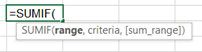
=SUMIF(range, criteria, [sum_range])
- The range parameter is actually the range of cells that will be evaluated by the ‘criteria’ parameter.
- The criteria parameter is the condition that must be met in the range parameter. For instance, if our range was a column that listed t-shirt color, a value like red or white could be our criteria. The criteria value can be text, a number, a date, a logical expression, a cell reference, or even another function.
- The sum_range parameter is optional as noted by the brackets. This simply means that if omitted, the sum_range will default to the same cells you chose for the ‘range’ parameter.
CountIF Function
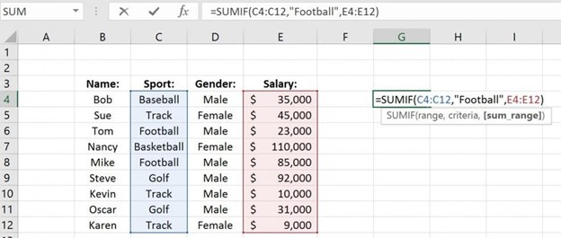
The Excel COUNTIF function in the Excel table determines the number of items, based on the criterion we provide. The function can be used, as an example, for determining the quantity of supplies, stocktaking, etc. The manual assumes that we have basic knowledge of creating formulas in Excel.
Use COUNTIF, one of the statistical functions, to count the number of cells that meet a criterion; for example, to count the number of times a particular city appears in a customer list. =COUNTIF(Where do you want to look?, What do you want to look for?)
Syntax =COUNTIF(range, criteria)
AverageIF Function
AVERAGEIF calculates central tendency, which is the location of the center of a group of numbers in a statistical distribution. Returns the average (arithmetic mean) of all the cells in a range that meet a given criteria.
Syntax =AVERAGEIF(range, criteria, [average_range])
Watch the full training
Watch the full training to learn advanced Excel techniques and best practices. You’ll get a quick overview of Excel’s advanced features and common business use cases. No matter what your experience with Excel is, you’ll leave this training with something new.