


Lookup functions in Excel simplify data retrieval by allowing users to search for specific information within datasets efficiently.
How to Use vLookup and xLookup Functions in Excel
vLookup
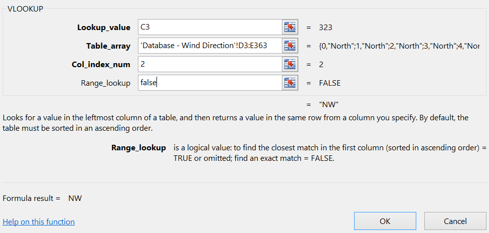
The V in VLOOKUP stands for “Vertical.” In Excel, the VLookup function searches for value in the left-most column of table_array and returns the value in the same row based on the index_number.
Usually lists like this have some sort of unique identifier for each item in the list. In this case, the unique identifier is in the “Item Code” column. Note: For the VLOOKUP function to work with a database/list, that list must have a column containing the unique identifier (or “key”, or “ID”), and that column must be the first column in the table. Our sample database above satisfies this criterion.
The secret to VLOOKUP is to organize your data so that the value you look up is to the left of the return value you want to find.
The VLOOKUP function syntax has the following arguments:
VLOOKUP (lookup_value, table_array, col_index_num, [range_lookup])
For example:
=VLOOKUP(105,A2:C7,2,TRUE)
=VLOOKUP(“Fontana”,B2:E7,2,FALSE)
lookup_value (required)
- The value you want to look up. The value you want to look up must be in the first column of the range of cells you specify in table-array.
- For example, if table-array spans cells B2:D7, then your lookup_value must be in column B. See the graphic below. Lookup_value can be a value or a reference to a cell.
table_array (required)
- The range of cells in which the VLOOKUP will search for the lookup_value and the return value.
- The first column in the cell range must contain the lookup_value (for example, Last Name in the picture below.) The cell range also needs to include the return value (for example, First Name in the graphic below) you want to find.
col_index_num (required)
- The column number (starting with 1 for the left-most column of table-array) that contains the return value.
range_lookup (optional)
- A logical value that specifies whether you want VLOOKUP to find an exact match or an approximate match:
- TRUE assumes the first column in the table is sorted either numerically or alphabetically, and will then search for the closest value. This is the default method if you don’t specify one.
- FALSE searches for the exact value in the first column.
XLookup
The XLOOKUP function searches a range or an array, and then returns the item corresponding to the first match it finds. If no match exists, then XLOOKUP can return the closest (approximate) match.
=XLOOKUP(lookup_value, lookup_array, return_array, [if_not_found], [match_mode], [search_mode])
Argument Description
lookup_value
(*required)The value to search for
(*If omitted, XLOOKUP returns blank cells it finds in lookup_array.)
lookup_array
(*required)The array or range to search
return_array
(*required)The array or range to return
[if_not_found]
(*optional)Where a valid match is not found, return the [if_not_found] text you supply.
If a valid match is not found, and [if_not_found] is missing, #N/A is returned.
[match_mode]
(*optional)Specify the match type:
0 - Exact match. If none found, return #N/A. This is the default.
-1 - Exact match. If none found, return the next smaller item.
1 - Exact match. If none found, return the next larger item.
2 - A wildcard match where *, ?, and ~ have special meaning
[search_mode]
(*optional)Specify the search mode to use:
1 - Perform a search starting at the first item. This is the default.
-1 - Perform a reverse search starting at the last item.
2 - Perform a binary search that relies on lookup_array being sorted in ascending order. If not sorted, invalid results will be returned.
-2 - Perform a binary search that relies on lookup_array being sorted in descending order. If not sorted, invalid results will be returned.
Examples:
Example 1 uses XLOOKUP to look up a country name in a range, and then return its telephone country code. It includes the lookup_value (cell F2), lookup_array (range B2:B11), and return_array (range D2:D11) arguments. It doesn’t include the match_mode argument, as XLOOKUP produces an exact match by default.
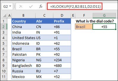
*Note: XLOOKUP uses a lookup array and a return array, whereas VLOOKUP uses a single table array followed by a column index number. The equivalent VLOOKUP formula in this case would be: =VLOOKUP(F2,B2:D11,3,FALSE)
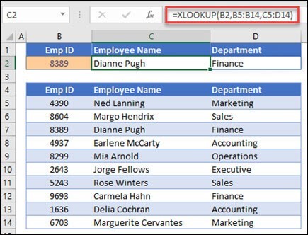
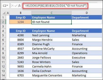
Example 2 looks up employee information based on an employee ID number. Unlike VLOOKUP, XLOOKUP can return an array with multiple items, so a single formula can return both employee name and department from cells C5:D14.
Example 3 adds an if_not_found argument to the preceding example.
Both formulas will return the same result. Notice, however, for XLOOKUP we provided both the lookup column and the result column separately. While for VLOOKUP we needed to provide the whole table and indicate the result column number. The additional difference we see is that in XLOOKUP we didn’t have to provide the exact match parameter – in XLOOKUP the default is an exact match.
This makes the XLOOKUP function a combination of INDEX & MATCH functions. The VLOOKUP had a lot of issues like having to put the lookup column at the front of the table or at least before the result column.
Watch the full training
Watch the full training to learn advanced Excel techniques and best practices. You’ll get a quick overview of Excel’s advanced features and common business use cases. No matter what your experience with Excel is, you’ll leave this training with something new.